Observations
The observation of agent is a 1D array consists with 5 parts. And the joint observation of the whole team is a 2D array, which is the stack version of all agents’ observations in the team.
Note
All entries in the observations are stored in float64, even if the actual values are integers. The observation spaces are continuous for both teams.
Camera Observations
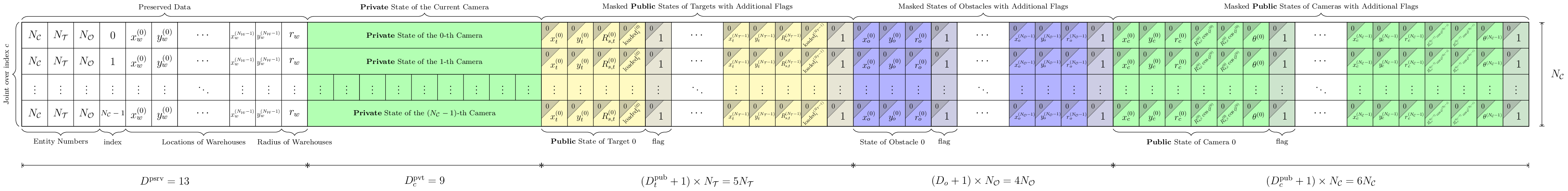
A camera observation \(\boldsymbol{o}_c\) consists of 5 parts:

Camera Observation
- The preserved part \(\boldsymbol{s}^{\text{prsv}}\) contains the some auxiliary information. And all values are constants during the whole episode.
observation[0](\(N_{\mathcal{C}}\))Number of cameras in the environment. This is a constant after
env.__init__().observation[1](\(N_{\mathcal{T}}\))Number of targets in the environment. This is a constant after
env.__init__().observation[2](\(N_{\mathcal{O}}\))Number of obstacles in the environment. This is a constant after
env.__init__().observation[3](\(c\))The index of the current camera in the team (in zero-based numbering). This is a constant after
env.reset().observation[4:12](\(x^{(0)}_w, y^{(0)}_w, \dots, x^{(N_{\mathcal{W}} - 1)}_w, y^{(N_{\mathcal{W}} - 1)}_w\))Locations of warehouses. They are constants.
observation[12](\(r_w\))Radius of warehouses. This is a constant.
- The private state of current camera (see Camera States).
observation[13:22](\(\boldsymbol{s}_c^{\text{pvt}}\))The private state of the current camera (i.e. the \(c\)-th camera, in zero-based numbering).
- Masked public states of targets with additional flags (see Target States).
A flag function defined as follows:
\[\operatorname{flag}^{(\text{C2T})} (c, t) = \mathbb{I} \left[ \text{the $t$-th target is track by the $c$-th camera} \right] \in \{ 0, 1 \},\]where \(c\) and \(t\) is the corresponding indices of the camera and the target in their team (in zero-based numbering).
A target is tracked by a camera when one of the following conditions is true:
The target is in the camera’s sector shaped field of view and not obscured by any obstacle.
If the target is in the camera’s sector shaped field of view but obscured by one or more obstacles, the target can be perceived with a probability. The probability is equal to the transmittance coefficient of obstacles defined by the configuration file.
If the current camera tracks the \(t\)-th target (i.e. \(\operatorname{flag}^{(\text{C2T})} (c, t) = 1\)):
observation[22 + 5 * t:22 + 5 * t + 4] (0 <= t < N_t)(\(\boldsymbol{s}_t^{\text{pub}}\))The public state of the \(t\)-th target.
observation[22 + 5 * t + 4] (0 <= t < N_t)(\(\operatorname{flag}^{(\text{C2T})} (c, t)\))One.
Otherwise (i.e. \(\operatorname{flag}^{(\text{C2T})} (c, t) = 0\)):
observation[22 + 5 * t:22 + 5 * t + 4] (0 <= t < N_t)Filled with zeros.
observation[22 + 5 * t + 4] (0 <= t < N_t)(\(\operatorname{flag}^{(\text{C2T})} (c, t)\))Zero.
- Masked states of obstacles with additional flags (see Obstacle States).
A flag function defined as follows:
\[\begin{split}\begin{split} \operatorname{flag}^{(\text{C2O})} (c, o) & = \mathbb{I} \left[ \text{the $o$-th obstacle can be sensed by the $c$-th camera} \right] \\ & = \begin{cases} 1, & {\left\| \vec{\boldsymbol{x}}_c^{(c)} - \vec{\boldsymbol{x}}_o^{(o)} \right\|}_2 \le R_{s,c,\max}^{(c)} + r_o^{(o)}, \\ 0, & \text{otherwise}. \end{cases} \end{split}\end{split}\]where \(c\) and \(o\) is the corresponding indices of the camera and the obstacle (in zero-based numbering) and \(\vec{\boldsymbol{x}} = (x, y)\). This flag function will be consistent during the whole episode.
If the current camera can sense the \(o\)-th obstacle (i.e. \(\operatorname{flag}^{(\text{C2O})} (c, o) = 1\)):
observation[22 + 5 * N_t + 4 * o:22 + 5 * N_t + 4 * o + 3] (0 <= o < N_o)(\(\boldsymbol{s}_o\))The state of the \(o\)-th obstacle.
observation[22 + 5 * N_t + 4 * o + 3] (0 <= o < N_o)(\(\operatorname{flag}^{(\text{C2O})} (c, o)\))One.
Otherwise (i.e. \(\operatorname{flag}^{(\text{C2O})} (c, o) = 0\)):
observation[22 + 5 * N_t + 4 * o:22 + 5 * N_t + 4 * o + 3] (0 <= o < N_o)Filled with zeros.
observation[22 + 5 * N_t + 4 * o + 3] (0 <= o < N_o)(\(\operatorname{flag}^{(\text{C2O})} (c, o)\))Zero.
- Masked public states of teammates (including itself for convenience) with additional flags (see Camera States).
A flag function defined as follows:
\[\begin{split} \operatorname{flag}^{(\text{C2C})} (c_1, c_2) & = \mathbb{I} \left[ \text{the $c_2$-th camera is perceived by the $c_1$-th camera} \right] \in \{ 0, 1 \}, \end{split}\]where \(c\) and \(c'\) is the corresponding indices of the cameras (in zero-based numbering). The logic of the flag function \(\operatorname{flag}^{(\text{C2C})}\) is same as \(\operatorname{flag}^{(\text{C2T})}\), i.e., within the camera’s sector shaped field of view and not occlude by any obstacle.
If the current camera perceives the \(d\)-th camera (i.e. \(\operatorname{flag}^{(\text{C2C})} (c, d) = 1\)):
observation[22 + 5 * N_t + 4 * N_o + 7 * d:22 + 5 * N_t + 4 * N_o + 7 * d + 6] (0 <= d < N_c)(\(\boldsymbol{s}_d^{\text{pub}}\))The public state of the \(s\)-th target.
observation[22 + 5 * N_t + 4 * N_o + 7 * d + 6] (0 <= d < N_c)(\(\operatorname{flag}^{(\text{C2C})} (c, d)\))One.
Otherwise (i.e. \(\operatorname{flag}^{(\text{T2T})} (t, s) = 0\)):
observation[22 + 5 * N_t + 4 * N_o + 7 * d:22 + 5 * N_t + 4 * N_o + 7 * d + 6] (0 <= d < N_c)Filled with zeros.
observation[22 + 5 * N_t + 4 * N_o + 7 * d + 6] (0 <= d < N_c)(\(\operatorname{flag}^{(\text{C2C})} (c, d)\))Zero.
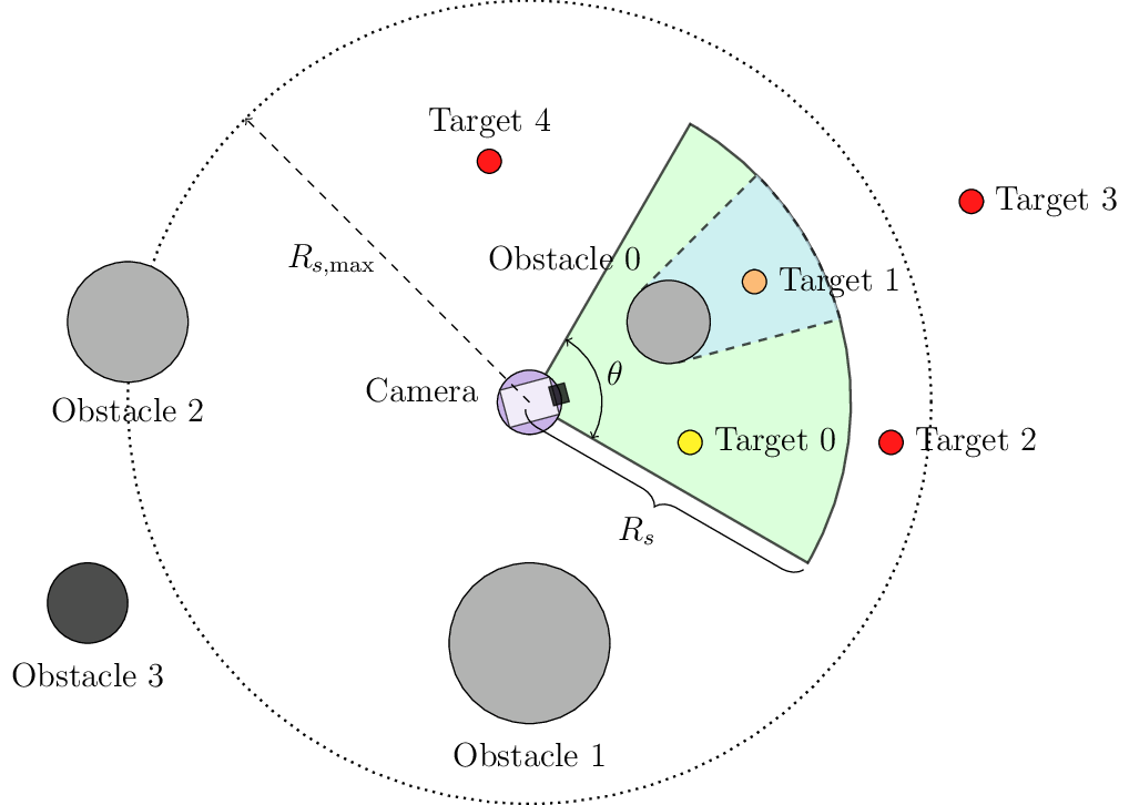
| [Camera (in purple)] | the camera's sector shaped field of view (in green) and the bind spot (in cyan) | |
| [Target] | tracked (in yellow), untracked (in red) and might be tracked with the probability of transmittance (in orange) | |
| [Obstacle] | sensed (in light gray) and not sensed (in darker gray) | |
| [Other Camera] | (not shown in the figure) the other camera can be sensed when in the camera's sector shaped field of view (same as the target) |
Note
For clarity, the targets are drawn as circles here. The actual radiuses of targets are \(0\).
The camera observation can be formulated as:
where \(\mathbb{C}\) means concatenation, \(\mathbb{F}\) is the flatten operation, and \(\otimes\) means element-wise multiplication. For the mask in each row, it’s a binary variable that indicates whether the entity is observable by the current camera.
The shape of a single camera observation is:
The joint version of camera observation is a 2D array, a stack of observations from all cameras. The shape of the joint observation is:
Joint Camera Observation
Target Observations
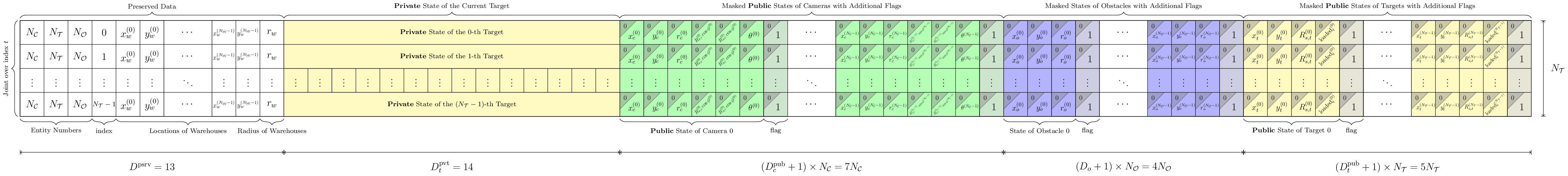
A target observation \(\boldsymbol{o}_t\) consists of 5 parts:

Target Observation
- The preserved part \(\boldsymbol{s}^{\text{prsv}}\) contains the some auxiliary information. And all values are constants during the whole episode.
observation[0](\(N_{\mathcal{C}}\))Number of cameras in the environment. This is a constant after
env.__init__().observation[1](\(N_{\mathcal{T}}\))Number of targets in the environment. This is a constant after
env.__init__().observation[2](\(N_{\mathcal{O}}\))Number of targets in the environment. This is a constant after
env.__init__().observation[3](\(t\))The index of the current target in the team (in zero-based numbering). This is a constant after
env.reset().observation[4:12](\(x^{(0)}_w, y^{(0)}_w, \dots, x^{(N_{\mathcal{W}} - 1)}_w, y^{(N_{\mathcal{W}} - 1)}_w\))Locations of warehouses. They are constants.
observation[12](\(r_w\))Radius of warehouses. This is a constant.
- The private state of current target (see Target States).
observation[13:27](\(\boldsymbol{s}_t^{\text{pvt}}\))The private state of the current target (i.e. the \(t\)-th target, in zero-based numbering).
- Masked public states of cameras with additional flags (see Camera States).
A flag function defined as follows:
\[\begin{split}\begin{split} \operatorname{flag}^{(\text{T2C})} (t, c) & = \mathbb{I} \left[ \text{the $c$-th camera is within the $t$-th target's sight range} \right] \\ & = \begin{cases} 1, & {\left\| \vec{\boldsymbol{x}}_t^{(t)} - \vec{\boldsymbol{x}}_c^{(c)} \right\|}_2 \le R_{s,t}^{(t)} + r_c^{(c)}, \\ 0, & \text{otherwise}. \end{cases} \end{split}\end{split}\]where \(c\) and \(t\) is the corresponding indices of the camera and the target in their team (in zero-based numbering) and \(\vec{\boldsymbol{x}} = (x, y)\). This flag function ignores any occlusion by obstacles.
If the current target perceives the \(c\)-th camera (i.e. \(\operatorname{flag}^{(\text{T2C})} (t, c) = 1\)):
observation[27 + 7 * c:27 + 7 * c + 6] (0 <= c < N_c)(\(\boldsymbol{s}_c^{\text{pub}}\))The public state of the \(c\)-th camera.
observation[27 + 7 * c + 6] (0 <= c < N_c)(\(\operatorname{flag}^{(\text{T2C})} (t, c)\))One.
Otherwise (i.e. \(\operatorname{flag}^{(\text{T2C})} (t, c) = 0\)):
observation[27 + 7 * c:27 + 7 * c + 6] (0 <= c < N_c)Filled with zeros.
observation[27 + 7 * c + 6] (0 <= c < N_c)(\(\operatorname{flag}^{(\text{T2C})} (t, c)\))Zero.
- Masked states of obstacles with additional flags (see Obstacle States).
A flag function defined as follows:
\[\begin{split}\begin{split} \operatorname{flag}^{(\text{T2O})} (t, o) & = \mathbb{I} \left[ \text{the $o$-th obstacle is within the $t$-th target's sight range} \right] \\ & = \begin{cases} 1, & {\left\| \vec{\boldsymbol{x}}_t^{(t)} - \vec{\boldsymbol{x}}_o^{(o)} \right\|}_2 \le R_{s,t}^{(t)} + r_o^{(o)}, \\ 0, & \text{otherwise}. \end{cases} \end{split}\end{split}\]where \(t\) and \(o\) is the corresponding indices of the camera and the obstacle (in zero-based numbering) and \(\vec{\boldsymbol{x}} = (x, y)\). This flag function ignores any occlusion by other obstacles.
If the current target senses the \(o\)-th obstacle (i.e. \(\operatorname{flag}^{(\text{T2O})} (t, o) = 1\)):
observation[27 + 7 * N_c + 4 * o:27 + 7 * N_c + 4 * o + 3] (0 <= o < N_o)(\(\boldsymbol{s}_o\))The state of the \(o\)-th obstacle.
observation[27 + 7 * N_c + 4 * o + 3] (0 <= o < N_o)(\(\operatorname{flag}^{(\text{T2O})} (t, o)\))One.
Otherwise (i.e. \(\operatorname{flag}^{(\text{T2O})} (t, o) = 0\)):
observation[27 + 7 * N_c + 4 * o:27 + 7 * N_c + 4 * o + 3] (0 <= o < N_o)Filled with zeros.
observation[27 + 7 * N_c + 4 * o + 3] (0 <= o < N_o)(\(\operatorname{flag}^{(\text{T2O})} (t, o)\))Zero.
- Masked public states of teammates (including itself for convenience) with additional flags (see Target States).
A flag function defined as follows:
\[\begin{split}\begin{split} \operatorname{flag}^{(\text{T2T})} (t_1, t_2) & = \mathbb{I} \left[ \text{the $t_2$-th target is perceived by the $t_1$-th target} \right] \\ & = \begin{cases} 1, & {\left\| \vec{\boldsymbol{x}}_t^{(t_1)} - \vec{\boldsymbol{x}}_t^{(t_2)} \right\|}_2 \le R_{s,t}^{(t_1)}, \\ 0, & \text{otherwise}. \end{cases} \end{split}\end{split}\]where \(t_1\) and \(t_2\) is the corresponding indices of the targets (in zero-based numbering) and \(\vec{\boldsymbol{x}} = (x, y)\). This flag function ignores any occlusion by obstacles.
If the current target senses the \(s\)-th target (i.e. \(\operatorname{flag}^{(\text{T2T})} (t, s) = 1\)):
observation[27 + 7 * N_c + 4 * N_o + 5 * s:27 + 7 * N_c + 4 * N_o + 5 * s + 4] (0 <= s < N_t)(\(\boldsymbol{s}_s^{\text{pub}}\))The public state of the \(s\)-th target.
observation[27 + 7 * N_c + 4 * N_o + 5 * s + 4] (0 <= s < N_t)(\(\operatorname{flag}^{(\text{T2T})} (t, s)\))One.
Otherwise (i.e. \(\operatorname{flag}^{(\text{T2T})} (t, s) = 0\)):
observation[27 + 7 * N_c + 4 * N_o + 5 * s:27 + 7 * N_c + 4 * N_o + 5 * s + 4] (0 <= s < N_t)Filled with zeros.
observation[27 + 7 * N_c + 4 * N_o + 5 * s + 4] (0 <= s < N_t)(\(\operatorname{flag}^{(\text{T2T})} (t, s)\))Zero.
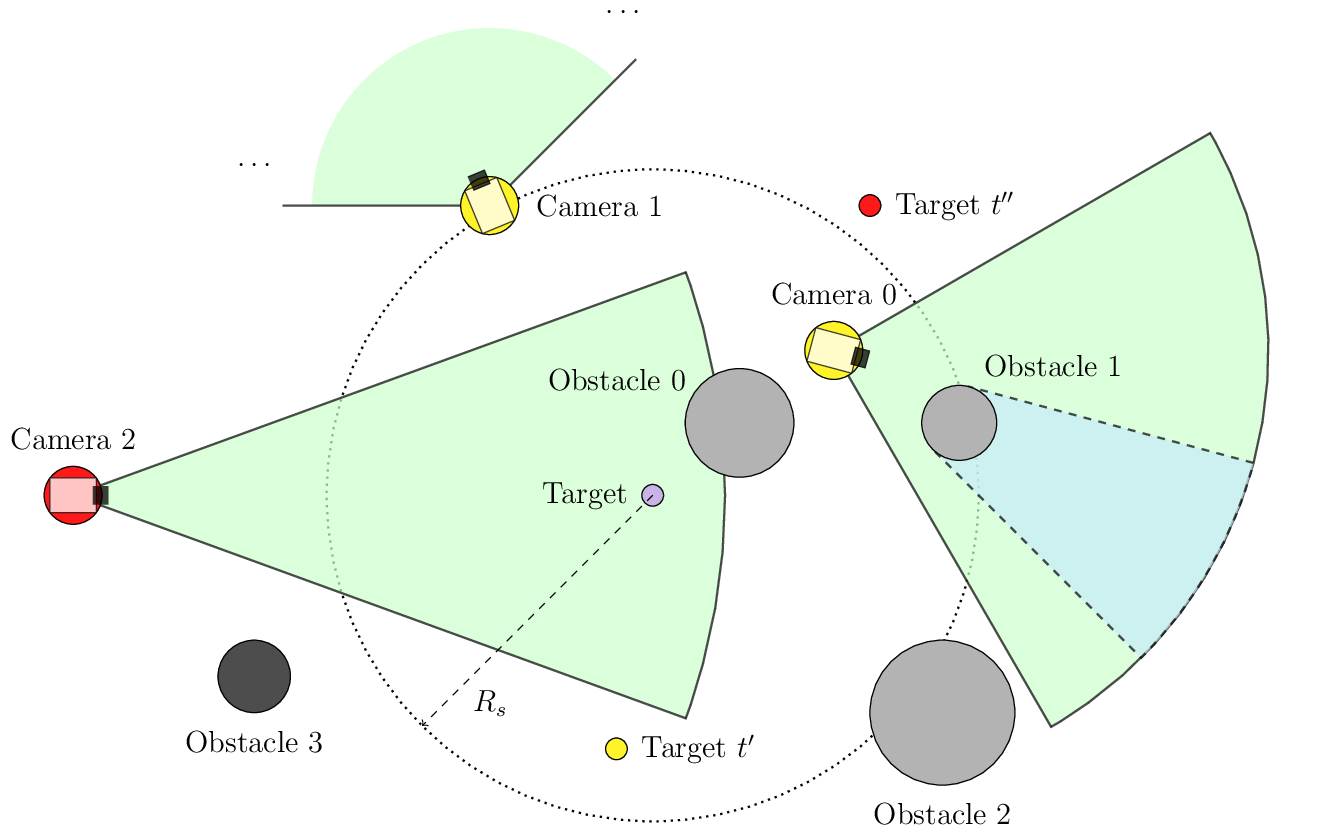
| [Target (in purple)] | the target's field of view (within dotted circle) | |
| [Camera] | perceived (in yellow), not perceived (in red) | |
| [Obstacle] | sensed (in light gray) and not sensed (in darker gray) | |
| [Other Target] | perceived (in yellow), not perceived (in red) |
Note
For clarity, the targets are drawn as circles here. The actual radiuses of targets are \(0\).
The target observation can be formulated as:
where \(\mathbb{C}\) means concatenation, \(\mathbb{F}\) is the flatten operation, and \(\otimes\) means element-wise multiplication. For the mask in each row, it’s a binary variable that indicates whether the entity is observable by the current target.
The shape of a single target observation is:
The joint version of target observation is a 2D array, a stack of observations from all targets. The shape of the joint observation is:
Joint Target Observation
- Related Resources